Feature Selection
Today’s datasets can consist of terabytes of data. It is not computationally feasible to train our model on all these parameters. Proper training does require a lot of data, don’t get me wrong, but not everything we have may be useful for our specific task. Neither is it memory-efficient to load all that data into 16 GB of memory. There are ways to handle this programmatically, such as using data loaders (PyTorch DataLoader or MONAI), but another option is to analyse the data statistically and determine whether each feature is significant. These techniques are called feature selection.
In this post, I will focus on some statistical techniques. In a future post, I may write some Python code to analyse real-world data, perhaps from the CERN Open Data Portal.
There are broadly three categories of feature selection. Today we look at filter-based methods.
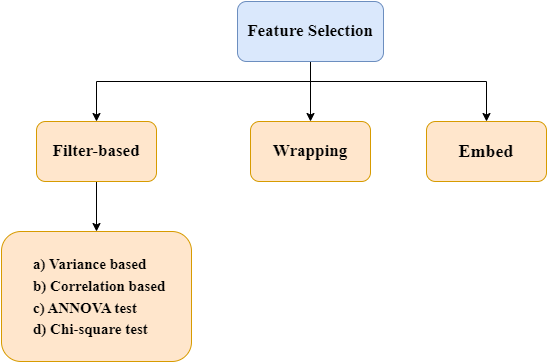
Filter-Based Techniques
Variance-Based Filtering
| Salary | Company |
|---|---|
| 1000 | A |
| 1000 | B |
| .. | .. |
| 1000 | C |
Let’s look at these columns for a bit. There is little to no variance in salary across companies A, B, and C. So, if I am to predict a company based on salary, the salary column gives me no useful information. The formula for calculating variance is:
So,
for each attribute:
     calculate the variance
Attributes with low variance can be rejected.
Limitation: This method only works for numeric data.
Correlation-Based Filtering
Correlation-based filtering, unlike the method above, works with two columns. Suppose there are two columns, A and B, as displayed below. If their correlation is above a certain threshold, we can reject either attribute A or attribute B because both then represent similar information.
| Day | A | B |
|---|---|---|
| 1 | 1.2% | 3.1% |
| 2 | 1.8% | 4.2% |
| 3 | 2.2% | 5.0% |
| 4 | 1.5% | 4.2% |
Formula
Correlation is related to covariance. The formula to calculate covariance between two attribute columns, A and B, is:
where μA is the mean of all the data in attribute A, and the same applies to μB. Here is a sample calculation:
Day 1=(1.2−1.675)×(3.1−4.125)=0.487
Day 2=(1.8−1.675)∗(4.2−4.125)=0.009
Day 3=(2.2−1.675)∗(5.0−4.125)=0.459
Day 4=(1.5−1.675)∗(4.2−4.125)=−0.013
Correlation = (0.487 + 0.009 + 0.459 − 0.013) / (4 − 1) = 0.943 / 3
Now all you need is a suitable threshold. If the correlation exceeds it, you reject one of the attributes.
Limitation: This method only works for numeric data. Sad, right? Don’t worry: ANOVA and the chi-square test are coming to your rescue!
ANOVA
| Companies( Non-numeric) | NumericData( Salary) |
|---|---|
| A | - |
| B | - |
| B | - |
| C | - |
Suppose we are given this dataset and want to know whether the company column affects the salary column. If it doesn’t, we can remove the company column altogether because an individual’s salary does not seem to be affected by the company. We calculate the mean and variance of salaries for each company using a metric called the F-score. A rough calculation of this metric is:
If the F-score is high, we infer that the company does have an impact on salary. Intuitively, this makes sense. We want low variance in salaries within a group; that is, people at a given company earn similar salaries, so the denominator (within-group variance) is small. We also want high variance between companies; changing companies produces different salaries, so the numerator (between-group variance) is large. The overall F-score is therefore high.
Let’s consider three companies—Amazon, TCS, and Bajaj—with n1 data points for TCS, n2 data points for Amazon, and n3 data points for Bajaj. We can calculate the within-group and between-group variance.
Within-group variance formula:

Between-group variance formula:
This is the full formula for the F-score:
Here, the variances are normalised by the degrees of freedom. DOFw represents the degrees of freedom within the group: the number of training data points minus the number of groups or classes. DOFb represents the degrees of freedom between groups: the number of groups minus one. For a chosen confidence level and the two degrees of freedom, we can look up a critical value in an F-distribution table. If the F-score is greater than that value, we say that company name has a statistically significant relationship with salary. We should therefore retain the company feature rather than remove it.
BOOM! ANOVA testing understood.
Limitation: What if there are multiple categorical attributes, such as company and designation? Stay tuned for the chi-square test!